Lab 4, CSC430, Spring 2022
1 Acknowledgments
This lab uses exercises (with permission) from a lab written by Kurt Voelker. Many thanks!
2 Exercises
In the exercises below, any instruction to "develop a function" implies the following steps:
Deciding what kind of data the function will accept (in future labs, you will have to make decisions about how the data will be structured),
Writing the first line of the function including the function name and parameter names,
Adding a docstring that indicates the purpose of the function,
Writing test cases for the function using assert, and finally
Writing the body of the function.
The monthly payment M of a loan amount P for y years with interest rate r can be calculated by the formula
M = \frac{(r/12)P}{1-(1 + r/12)^{-12y}}
Develop the monthly_payment function, that accepts loan amount, years, and annual rate, and returns the monthly payment using the formula above.
Hint: make sure you’re setting r correctly, do some sanity testing.
Develop the total_payments function, that accepts the monthly payment and the number of years and returns the total of all payments, assuming 12 months per year.
Using these functions, calculate the monthly payment and the total payment for a $100,000 loan for 10, 11, ... , 29, 30 years with an interest rate of 4.85%. Construct a NumPy array and display the results in a three-column table where the first column is the number of years, the second is the monthly payment, and the third is the total payment (that is, the sum of the payments over the life of the loan).
A railroad bumper is designed to slow down a rapidly moving railroad car. After a 20,000 kg railroad car traveling at 20 m/s engages the bumper, its displacement x (in meters) and velocity v (in m/s) as a function of time t (in seconds) is given by x(t) = 4.219(e^{-1.58t}-e^{-6.32t}) and v(t) = 26.67e^{-6.32t}-6.67e^{-1.58t}
Here’s a picture!
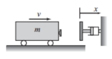
Develop the functions bumper_x and bumper_v that accept the time in seconds and return the displacement and the velocity respectively.
Use these functions to compute a NumPy array representing a three-column table in which the first column is time (in seconds), the second is displacement (in meters), and the third is velocity (in m/s).
Show the values for every two-hundredth of a second for the first half-second after impact.
- The vapor pressure p (in units of mm Hg) of benzene with temperature in the range of 0 \leq T \leq 42°C can be modeled with the equation
from Handbook of Chemistry and Physics, CRC Press
log_{10}p = b - \frac{0.05223a}{T} where a = 34172 and b = 7.9622 are material constants and T is absolute temperature (K).Develop the function benzene_pressure that accepts a temperature in degrees celsius (°C) and computes the vapor pressure of benzene using the formula above.
Using the benzene_pressure function, construct a NumPy array that displays as a table showing the temperatures from 0°C to 42°C, in increments of 2°C, and shows the corresponding pressure in mm Hg.